

Edge-oriented Convolution Block for Real-time Super Resolution on Mobile Devices (ECB)
1.abstract
This paper proposes a re-parameterizable building block for efficient super-resolution (SR), called the Edge-oriented Convolution Block (ECB). Most existing studies focus on reducing model parameters and FLOPs, but this does not necessarily improve runtime speed on mobile devices. ECB extracts features through multiple paths, including standard 3×3 convolution, channel expansion and compression convolutions, as well as first-order and second-order spatial derivatives derived from intermediate features. During the inference stage, these multiple operations can be merged into a single 3×3 convolution.
2.method
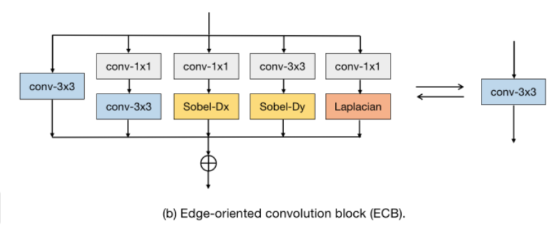
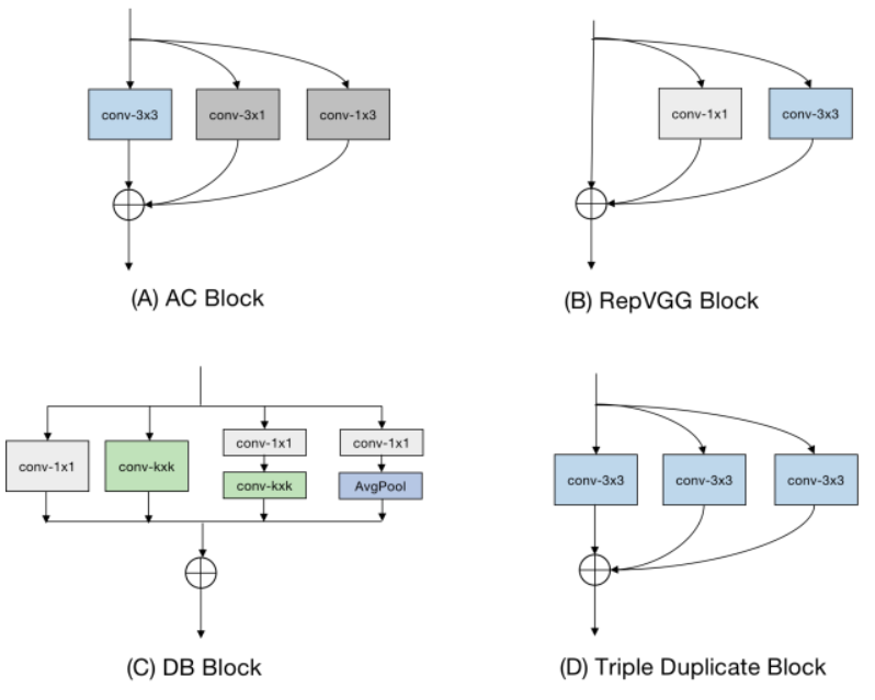
To improve the performance of super-resolution algorithms, the authors propose a re-parameterizable block called the Edge-oriented Convolution Block (ECB). Compared with previously applied re-parameterization blocks, ECB is more effective at extracting edge and texture information required for SR tasks, thereby enhancing the performance of the base model. The underlying technique of this paper is derived from [1], which describes how to simplify the sequential connection of a 1×1 convolution layer and a 3×3 convolution layer into a single convolution layer with a kernel size of 3.
Understanding Basic Parallel Convolution Fusion Technology
The figure below shows a flowchart of a standard 1×1 convolution layer.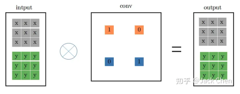 However, the above process can also be equivalently represented as the 3×3 convolution kernel operation shown in the figure below. The method is simple: just pad zeros around the original numbers. After this modification, the original 1×1 convolution kernel can be transformed into a 3×3 convolution kernel.
 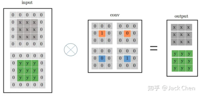 Two parallel convolution kernels can be combined into an equivalent convolution kernel according to the following formula. Assume the first 3×3 convolution kernel has weights \( k_0,b_0 \), and the second 3×3 convolution kernel has weights
  with input X
XX. Based on the process, the output can be derived as follows:\(O=(X*k_0+b_0)+(X*k_1+b_1)=(k_0+k_1)X+(b_0+b_1) \)
Thus, the new convolution kernel weights can now be obtained.
\(k_{new}=k_0+k_1 \)
\(b_{new}=b_0+b_1 \)
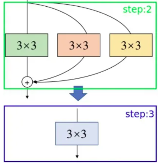 –
– - However, the connection method used in this paper is sequential, so the formula is derived as follows:
- \(O=(X*k_0+b_0)*k_1+b_1=k_0k_1X+b_0k_1+b_1\)
- Thus, the new convolution kernel weights can now be obtained.
- \(k_{new}=k_0k_1\)
- \(b_{new}=b_0k_1+b_1\)
- he complete code can be found in the official source release; a partial excerpt is shown below.
# conv1X1: self.k0,self.b0
# conv3X3: self.k1,self.b1

if self.type == 'conv1x1-conv3x3':
    # re-param conv kernel
    RK = F.conv2d(input=self.k1, weight=self.k0.permute(1, 0, 2, 3))
    # re-param conv bias
    RB = torch.ones(1, self.mid_planes, 3, 3, device=device) * self.b0.view(1, -1, 1, 1)
    RB = F.conv2d(input=RB, weight=self.k1).view(-1,) + self.b1
I also wrote a verification program myself to demonstrate that the two are indeed equivalent. A reference snippet is shown below.
import torch
import torch.nn as nn
import torch.nn.functional as F

class TestConv:
    def __init__(self):
        self.type = 'conv1x1-conv3x3'
        self.mid_planes = 16 # Example value
        self.k0 = torch.randn(self.mid_planes, 3, 1, 1)
        self.b0 = torch.randn(self.mid_planes)
        self.k1 = torch.randn(self.mid_planes, self.mid_planes, 3, 3)
        self.b1 = torch.randn(self.mid_planes)

    def reparameterize(self, device):
        # Re-param conv kernel
        RK = F.conv2d(input=self.k1, weight=self.k0.permute(1, 0, 2, 3))
        # Re-param conv bias
        RB = torch.ones(1, self.mid_planes, 3, 3, device=device) * self.b0.view(1, -1, 1, 1)
        RB = F.conv2d(input=RB, weight=self.k1).view(-1,) + self.b1
        return RK, RB

# Random input
input_tensor = torch.randn(1, 3, 8, 8)
test_conv = TestConv()

# Regular 1x1 and 3x3 convolutions
conv1x1 = nn.Conv2d(in_channels=3, out_channels=16, kernel_size=1)
conv3x3 = nn.Conv2d(in_channels=16, out_channels=16, kernel_size=3)
conv1x1.weight.data = test_conv.k0
conv1x1.bias.data = test_conv.b0
conv3x3.weight.data = test_conv.k1
conv3x3.bias.data = test_conv.b1

output_regular = conv3x3(conv1x1(input_tensor))

# Reparameterized convolution

RK, RB = test_conv.reparameterize(input_tensor.device)
conv_reparam = nn.Conv2d(in_channels=3, out_channels=16, kernel_size=3)
conv_reparam.weight.data = RK
conv_reparam.bias.data = RB

output_reparam = conv_reparam(input_tensor)

# Check if the outputs are close
assert torch.allclose(output_regular, output_reparam, atol=1e-5), "The outputs are not close!"
print("Test passed!")
3.experiments result
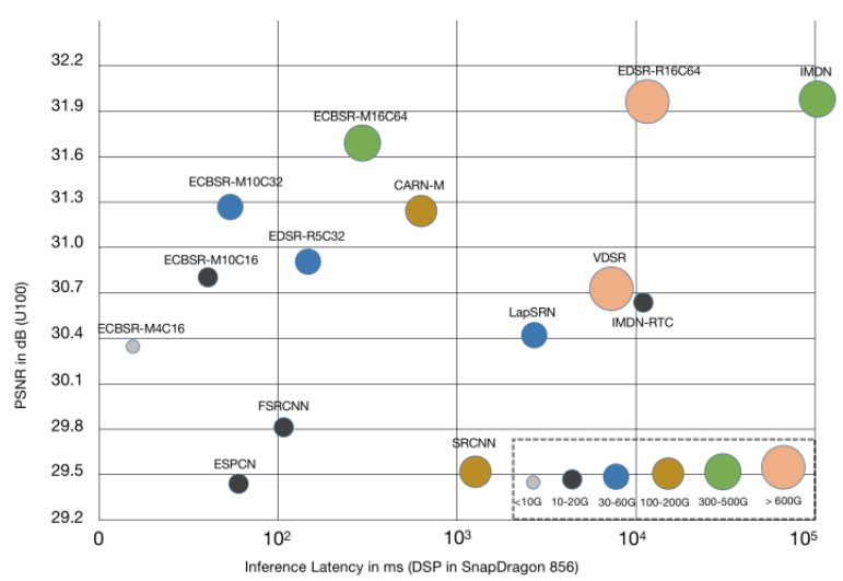
The authors compared their method with other re-parameterization models and found that the proposed ECB achieved the best performance across five public datasets. They also analyzed the impact of each individual component on the experimental results. From the experimental tables, it can be seen that combining all components yields the best overall effect.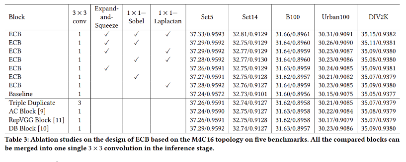 The authors also applied this network architecture to several SR models, where “+” indicates models enhanced with ECB. From the experimental results, it can be observed that both models achieved improvements across five public datasets after adopting the ECB architecture. This demonstrates that the proposed design effectively enhances network performance without adding any extra parameters or computational cost.
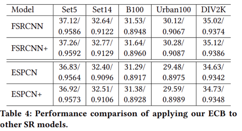 下The figure shows a visual comparison of the different models.
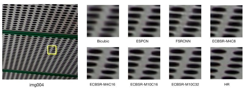
4.reference
RepVGG: Making VGG-style ConvNets Great Again
Diverse Branch Block: Building a Convolution as an Inception-like Unit